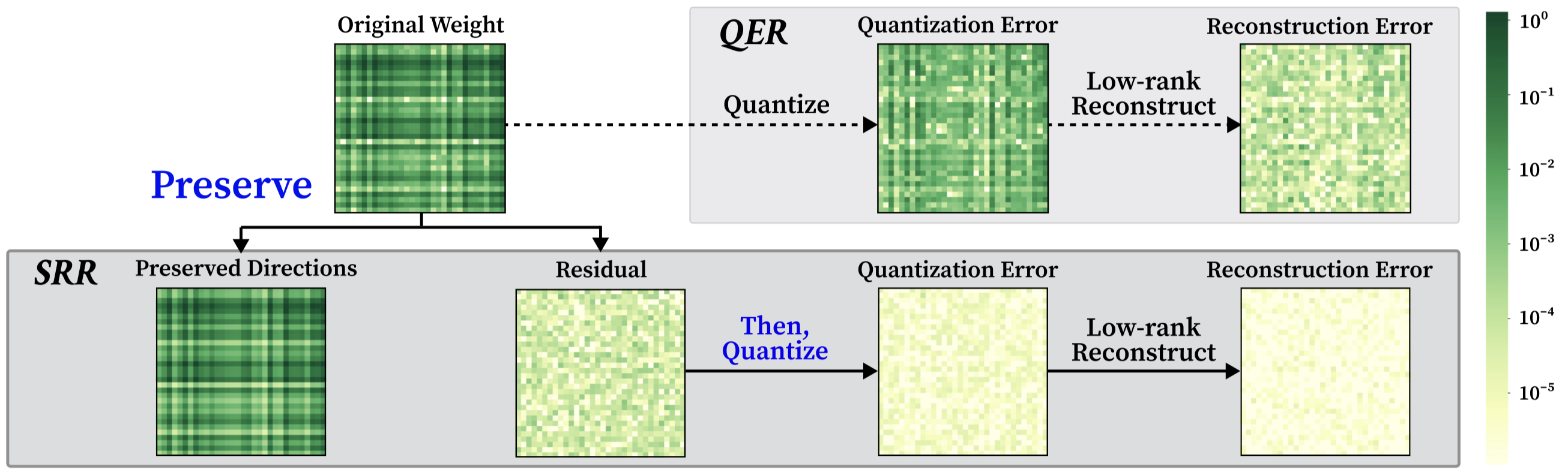
Preserve-Then-Quantize:
Balancing Rank Budgets for Quantization Error Reconstruction in LLMs

1Department of Computer Science, Yonsei University
2Department of Artificial Intelligence, Yonsei University
* Equal contribution; † Corresponding author.
ICML 2026

TL;DR: SRR improves QER & QPEFT by splitting the rank budget
between preserving dominant structure and reconstructing quantization error,
guided by a principled, cheap selection criterion.

SRR overview: preserve-then-quantize pipeline. Top: standard QER quantizes all of W. Bottom: SRR preserves the dominant subspace of SW before quantization, then reconstructs the residual.
Figure 1. Preserve-then-quantize in SRR vs. standard QER. QER (top) quantizes the full weight matrix, destroying its low-rank structure so that the residual error escapes any low-rank correction. SRR (bottom) preserves the dominant subspace before quantization, yielding a substantially smaller reconstruction error $\lVert \mathbf{W} - \mathbf{Q} - \mathbf{L}\mathbf{R} \rVert_F$ under the same rank budget.

Introduction

Post-Training Quantization (PTQ) is the standard technique for reducing the memory and inference cost of large language models (LLMs), but it degrades model accuracy. Quantization Error Reconstruction (QER) recovers this accuracy by augmenting the quantized weight matrix $\mathbf{Q}$ with a rank-$r$ correction $\mathbf{LR}$:

$$ \mathbf{W} \;\approx\; \mathbf{Q} + \mathbf{LR},\qquad \mathbf{L}\in\mathbb{R}^{m\times r},\ \mathbf{R}\in\mathbb{R}^{r\times n},\ r \ll \min(m,n). $$

Existing QER methods commit the entire rank budget $r$ to fitting the (scaled) residual $\mathbf{S}(\mathbf{W}-\mathbf{Q})$, implicitly assuming this residual is low-rank. The assumption breaks in low-bit regimes: the residual is dense and high-rank, while $\mathbf{SW}$ is highly anisotropic — most of its energy concentrates in a few dominant singular directions. Quantizing those dominant directions injects a disproportionately large error that a rank-limited correction then has to spend its capacity repairing.

We propose Structured Residual Reconstruction (SRR) (see Figure 1.), a preserve-then-quantize framework that explicitly splits the rank budget into two roles: $k$ ranks preserve the dominant subspace of $\mathbf{SW}$ before quantization, and the remaining $r-k$ ranks reconstruct the residual error afterwards. Choosing $k$ naively would require sweeping all values from $1$ to $r$ and selecting the one that minimizes the reconstruction error, resulting in $r$ full quantization passes per layer. This is prohibitively expensive. Instead, we derive a theory-guided criterion that selects $k$ in one shot, separately for each layer and each weight matrix.

Structured Residual Reconstruction (SRR)

The SRR Pipeline

Given a rank budget $r$ and a split $k\in\{0,\ldots,r\}$, SRR proceeds in three steps:

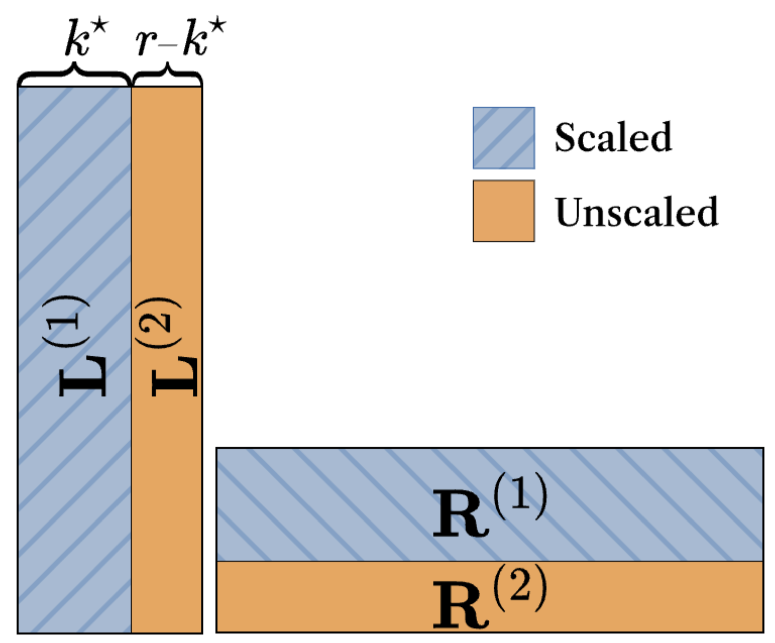
  1. Preserve. Take the top-$k$ singular components of the scaled weight $\mathbf{SW}$ and map them back to the original space:
    $$ \mathbf{L}_k^{(1)}\mathbf{R}_k^{(1)} \;:=\; \mathbf{S}^{-1}\,\mathrm{SVD}_k(\mathbf{SW}). $$
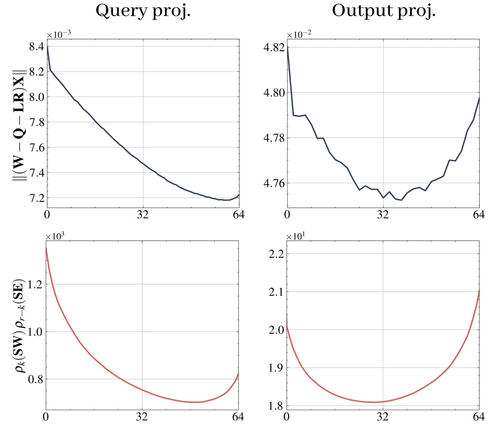
  2. Quantize the residual. Apply the base quantizer $\mathcal{Q}$ to what remains, and let $\mathbf{E}_k$ denote the resulting error:
    $$ \mathbf{Q}_k \;:=\; \mathcal{Q}\bigl(\mathbf{W}-\mathbf{L}_k^{(1)}\mathbf{R}_k^{(1)}\bigr),\qquad \mathbf{E}_k \;:=\; \mathbf{W}-\mathbf{L}_k^{(1)}\mathbf{R}_k^{(1)}-\mathbf{Q}_k. $$
  3. Reconstruct. Use the remaining $r-k$ ranks to fit the quantization error $\mathbf{E}_k$ in the scaled space:
    $$ \mathbf{L}_k^{(2)}\mathbf{R}_k^{(2)} \;:=\; \mathbf{S}^{-1}\,\mathrm{SVD}_{r-k}(\mathbf{SE}_k). $$

The final approximation $\widehat{\mathbf{W}}_{\mathrm{SRR}}(k) = \mathbf{L}_k^{(1)}\mathbf{R}_k^{(1)} + \mathbf{Q}_k + \mathbf{L}_k^{(2)}\mathbf{R}_k^{(2)}$ folds into the standard QER form $\widehat{\mathbf{W}} = \mathbf{Q} + \mathbf{LR}$.
SRR is therefore drop-in compatible with any quantizer and preserves the standard QER formulation.

How should we choose optimal $k$?

We want to choose $k$ that minimizes the scaled reconstruction error $\mathcal{L}(k) = \|\mathbf{S}(\mathbf{W} - \widehat{\mathbf{W}}_{\mathrm{SRR}}(k))\|_F$. As a first step, $\mathcal{L}(k)^2$ admits a clean two-factor form that exposes the trade-off:

$$ \mathcal{L}(k)^2 \;=\; \underbrace{\|\mathbf{SE}_k\|_F^2}_{\text{(1) scale}}\;\cdot\; \underbrace{\rho_{r-k}(\mathbf{SE}_k)}_{\text{(2) spectral}}, $$

where $\rho_p(\mathbf{A}):=\|\mathbf{A}-\mathrm{SVD}_p(\mathbf{A})\|_F^2/\|\mathbf{A}\|_F^2$ is the fraction of energy unrecoverable by the best rank-$p$ approximation.

  • (1) Scale: how much energy enters the quantizer. The first $k$ components of $\mathbf{SW}$ bypass quantization, so larger $k$ shrinks $\|\mathbf{SE}_k\|_F$. Favors large $k$.
  • (2) Spectral: what fraction of that error survives the best rank-$(r-k)$ correction. More remaining ranks absorb the error. Favors small $k$.
Top: reconstruction error |W - Q - LR|_F^2 as a function of k for the query and output projections. Bottom: surrogate ρ_k(SW) ρ_{r-k}(SE). Both are minimized at the same k*.
Figure 2. True reconstruction error (top) and our surrogate $\rho_k(\mathbf{SW})\rho_{r-k}(\mathbf{SE})$ (bottom). LLaMA-2 7B, layer 10, $r=64$.

This clarifies why $k$ must balance two opposing forces, but both factors still depend on $k$ through $\mathbf{E}_k$, so evaluating it for any candidate still needs quantization. We remove this with two mild assumptions that involve only the quantizer and bitwidth, not $k$:

  1. Assumption 4.1 (constant relative scale): for a fixed quantizer, $\|\mathbf{S}\,E_\mathcal{Q}(\mathbf{A})\|_F \approx \eta_\mathcal{Q}\,\|\mathbf{SA}\|_F$. This collapses the scale term to a quantity computable from $\mathbf{SW}$ alone: $\|\mathbf{SE}_k\|_F^2 \approx \eta_\mathcal{Q}^2\,\rho_k(\mathbf{SW})\,\|\mathbf{SW}\|_F^2$.
  2. Assumption 4.2 (spectral proxy): the normalized quantization residual behaves like unstructured noise after rounding, so $\rho_{r-k}(\mathbf{SE}_k) \approx \rho_{r-k}(\mathbf{SE})$ for a single random matrix probe $\mathbf{E}$. The spectral term is now decoupled from the actual residual.

Plugging both assumptions into the two-factor form yields a fully tractable surrogate:

$$ \mathcal{L}(k)^2 \;\approx\; \underbrace{\eta_\mathcal{Q}^2\,\|\mathbf{SW}\|_F^2\ \rho_k(\mathbf{SW})}_{\substack{\text{Asm. 4.1}}}\, \cdot\; \underbrace{\rho_{r-k}(\mathbf{SE})}_{\substack{\text{Asm. 4.2}}}. $$

Both factors are now computable from a single SVD each — one on the $\mathbf{SW}$, the other on a random probe $\mathbf{SE}$ — without ever touching the quantizer. Since $\eta_\mathcal{Q}$ and $\|\mathbf{SW}\|_F$ are constants in $k$, they drop out, leaving a closed-form, one-shot selection rule:

$$ k^\star \;=\; \arg\min_{0\le k\le r}\; \rho_k(\mathbf{SW})\,\rho_{r-k}(\mathbf{SE}). $$

Evaluating $k^\star$ now costs only two SVDs per layer — no enumeration over $k$, no repeated quantizations.
In practice, the surrogate tracks the true reconstruction error well as shown in Figure 2.

Extending SRR to QPEFT

SRR also yields a high-fidelity initialization for Quantized Parameter-Efficient Fine-Tuning (QPEFT): freezing $\mathbf{Q}$ and training only $\mathbf{LR}$ inherits the SRR decomposition. The two components carry very different magnitudes — $\mathbf{L}^{(1)}\mathbf{R}^{(1)}$ sits on the dominant subspace of $\mathbf{SW}$ with large singular values, while $\mathbf{L}^{(2)}\mathbf{R}^{(2)}$ fits a much smaller quantization residual — so a uniform learning rate either over-rotates the preserved subspace. We address this with gradient scaling: attenuate updates on the preserved factors by $\gamma\in(0,1)$, leaving the residual factors unscaled:

$$\nabla_{\mathbf{L}^{(1)}\mathbf{R}^{(1)}}\mathcal{L} \;\leftarrow\; \gamma\,\nabla_{\mathbf{L}^{(1)}\mathbf{R}^{(1)}}\mathcal{L}.$$

Coarse choices $\gamma\in\{0.1,0.5\}$ both work — gains come primarily from the better initialization, with gradient scaling serving as a simple regularizer against drift in the preserved subspace.

Left: singular-value spectrum of the SRR decomposition with the selected k* marked. Right: schematic of the two-component adapter, with the preserved block (L^(1), R^(1)) shaded as 'scaled' and the residual block (L^(2), R^(2)) shown as 'unscaled'.
Figure 3: Illustration of SRR for QPEFT. The first $k^\star$ columns/rows are gradient-scaled; the remaining $r-k^\star$ are left unscaled.

Experimental Results

Post-Training Quantization (PTQ)

Table 1: WikiText2 perplexity under 3-bit MXINT quantization at r=32 and r=64 across TinyLLaMA 1.1B, Gemma-2 2B, LLaMA-2 7B/13B, LLaMA-3.1 8B/70B. SRR is applied on top of LQER, QERA-approx, and QERA-exact, and is lowest in nearly every cell.
Perplexity ↓. Applied on top of three QER baselines (LQER, QERA-approx, QERA-exact), SRR consistently reduces WikiText2 perplexity under 3-bit MXINT — up to 12.2% on Gemma-2 2B, 27.1% on LLaMA-2 7B, and 3.6% on LLaMA-3.1 8B.
Table 2: Average zero-shot accuracy across five downstream tasks (HellaSwag, Winogrande, BoolQ, MMLU, BBH) at 3-bit MXINT, r=64. QERA-exact + SRR wins on every model size.
Zero-shot accuracy ↑. Even on top of the strong QERA-exact closed-form baseline, SRR still provides additional headroom across five downstream tasks — confirming there is structure beyond optimal residual fitting that a balanced rank split captures.
Table 5: WikiText2 perplexity with 3-bit GPTQ and 2-bit QuIP# quantizers on LLaMA-2 7B and LLaMA-3.1 8B. SRR improves every QER baseline under both quantizers.
Quantizer-agnostic. SRR transfers cleanly to activation-aware quantizers — both 3-bit GPTQ and 2-bit QuIP# see consistent perplexity drops.

Quantized Parameter-Efficient Fine-Tuning (QPEFT)

Table 3: GLUE fine-tuning results with RoBERTa-base under 4/3/2-bit MXINT. SRR achieves the best average across all bitwidths and the gap grows at lower precision.
GLUE / RoBERTa-base. SRR delivers the best average across 4/3/2-bit settings, with gains of +1.5 / +4.7 / +5.9 pp over QERA respectively — and over +10 pp versus LQ-LoRA at 2 bits.
Table 4: SlimPajama perplexity (r=8) and GSM8K accuracy (r=64) on LLaMA-2 7B and LLaMA-3.1 8B at 4-bit and 2-bit MXINT. SRR wins every cell.
SlimPajama + GSM8K. SRR cuts SlimPajama perplexity and lifts GSM8K accuracy across both LLaMA-2 7B and LLaMA-3.1 8B — especially at 2-bit, where baselines collapse.
Figure 4: Training loss curves on STSB (left) and CoLA (right) over five epochs for QLoRA, LoftQ, QERA, LQ-LoRA and SRR. SRR descends fastest and reaches the lowest loss.
Faster convergence. Beyond final accuracy, SRR's initialization yields visibly faster training-loss reduction on GLUE tasks — a direct consequence of starting from a high-fidelity $\mathbf{W}\approx\mathbf{Q}+\mathbf{LR}$ factorization.

BibTeX

@inproceedings{cho2026preserve,
  title={Preserve-Then-Quantize: Balancing Rank Budgets for Quantization Error Reconstruction in LLMs},
  author={Cho, Yoonjun and Jeon, Dongjae and Kim, Soeun and Jeon, Moongyu and No, Albert},
  journal={International Conference on Machine Learning},
  year={2026}
}